Modeling processors in gem5

Let’s start digging into the first of the three main categories of gem5 components: processors.

By the end of this section, you will be able to:

• Compare the features and advantages of simple, KVM, O3, and minor CPUs.
• Modify a processor by changing the CPU type.
• Change a CPU’s parameters by extending an existing CPU model in Python.
• Contrast the simulation behavior of atomic, functional, and timing memory accesses.
• Compare the simulation performance of different gem5 CPU types.

Processors in the standard library

Processors

In the previous section on the standard library, we mentioned that two types of processors exist: SimpleProcessor and SwitchableProcessor. Traffic generators, which pretend to be processors, can be used in their place.

• A SimpleProcessor is the general-purpose processor in the standard library, which lets you define its ISA, number of cores, and type (more on this in a minute!)
• A SwitchableProcessor is similar to a SimpleProcessor, but it allows switching between multiple types of processors during a simulation instead of using just one SimpleProcessor.
  • We’ll use a switchable processor during our advanced section on KVM fast-forwarding!
• Traffic generators are not really processors; they take the spot of a processor on a board, but they don’t execute instructions. Instead, they use traffic patterns (linear, random, etc.) to synthetically generate memory accesses. They’re ideal for testing cache hierarchies/memory systems.
  • We’ll use traffic generators in the intermediate features unit’s section on traffic generation!

Cores

Within every processor, there are one or more cores. The gem5 standard library provides core components that its processors (and, eventually, your own processors) can use! The cores follow a similar pattern to the processors:

• SimpleCore is the core used in all “regular” processors (SimpleProcessor and SwitchableProcessor).
• There are many types of generator cores, all of which extend from AbstractGeneratorCore. These are used in traffic generators.
  • Some examples include ComplexGeneratorCore, RandomGeneratorCore, etc.

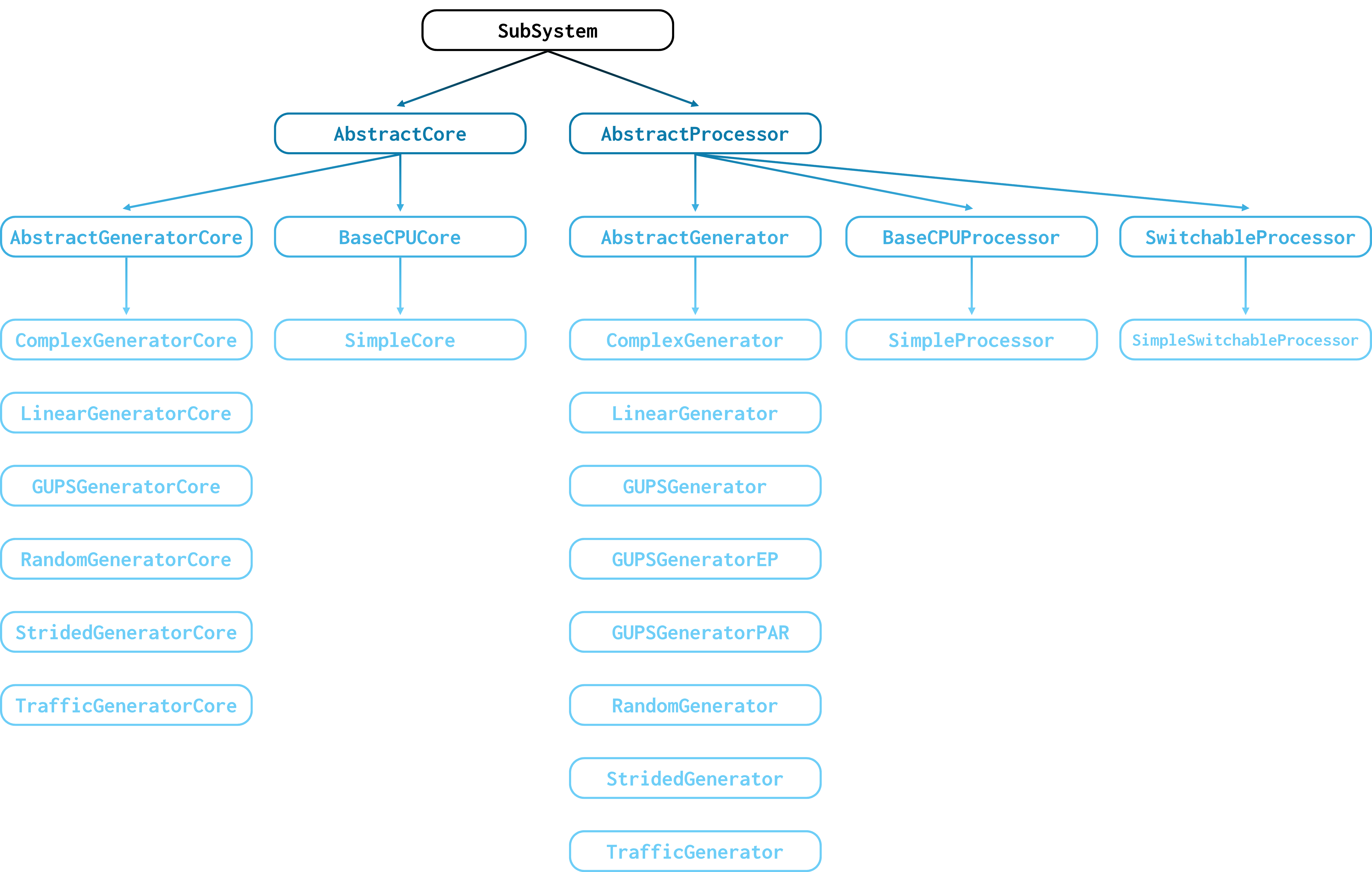
If you’re curious, the class diagram for every processor and core in the standard library is below.

src/python/gem5/components/processors

Using standard library processors

As we’ve discussed already, we can use standard library processors in the same way that we use all other standard library components: by instantiating them with our desired parameters and plugging them into our board. For example, in the previous section, we used a SimpleProcessor for our board like this:

# instantiate and set parameters
processor = SimpleProcessor(
  cpu_type = CPUTypes.TIMING,
  isa = ISA.X86,
  num_cores = 1
)

# plug into board
board = X86Board(
  ...
  processor = processor
)

You might notice, however, that we have yet to explain what cpu_type refers to. This is how we configure what CPU model the processor’s cores use.

CPU models in gem5

The standard library gives us an easy interface for processors and cores through components like SimpleProcessor, SwitchableProcessor, SimpleCore, and the array of available synthetic traffic generators/cores. Under the hood, these standard library components utilize gem5’s CPU models for their cores.

Remember that a component refers to a pre-defined standard library object written in Python. A model is a simulated object written in C++. gem5 has hundreds of models!

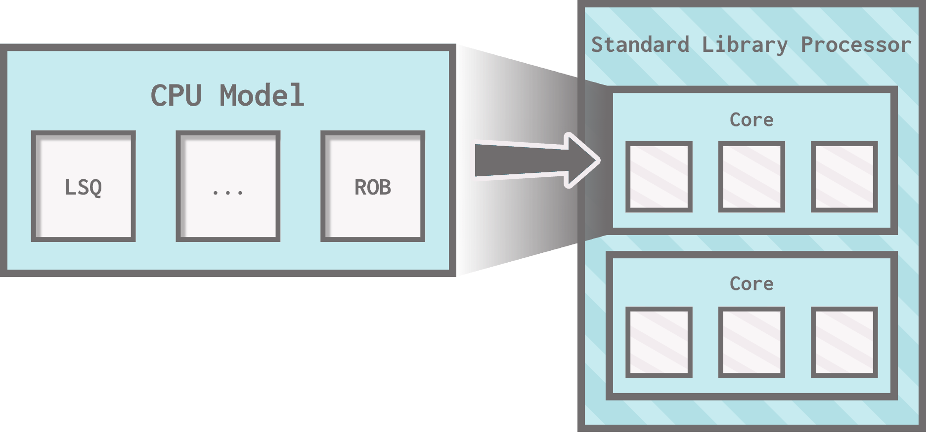
gem5 has five major CPU models:

• AtomicSimpleCPU (CPUTypes.ATOMIC)
• TimingSimpleCPU (CPUTypes.TIMING)
• KvmCPU (CPUTypes.KVM)
• MinorCPU (CPUTypes.MINOR)
• O3CPU (CPUTypes.O3)

Let’s discuss these CPU types in more detail.

Atomic and Timing Simple CPUs

A SimpleCPU (not to be confused with SimpleProcessor, the standard library processor component) is quite fast to simulate and has limited branch prediction capabilities.

As a reminder, branch prediction is a CPU’s ability to execute instructions after a branch (AKA jump) instruction by guessing whether the branch will be taken or not.

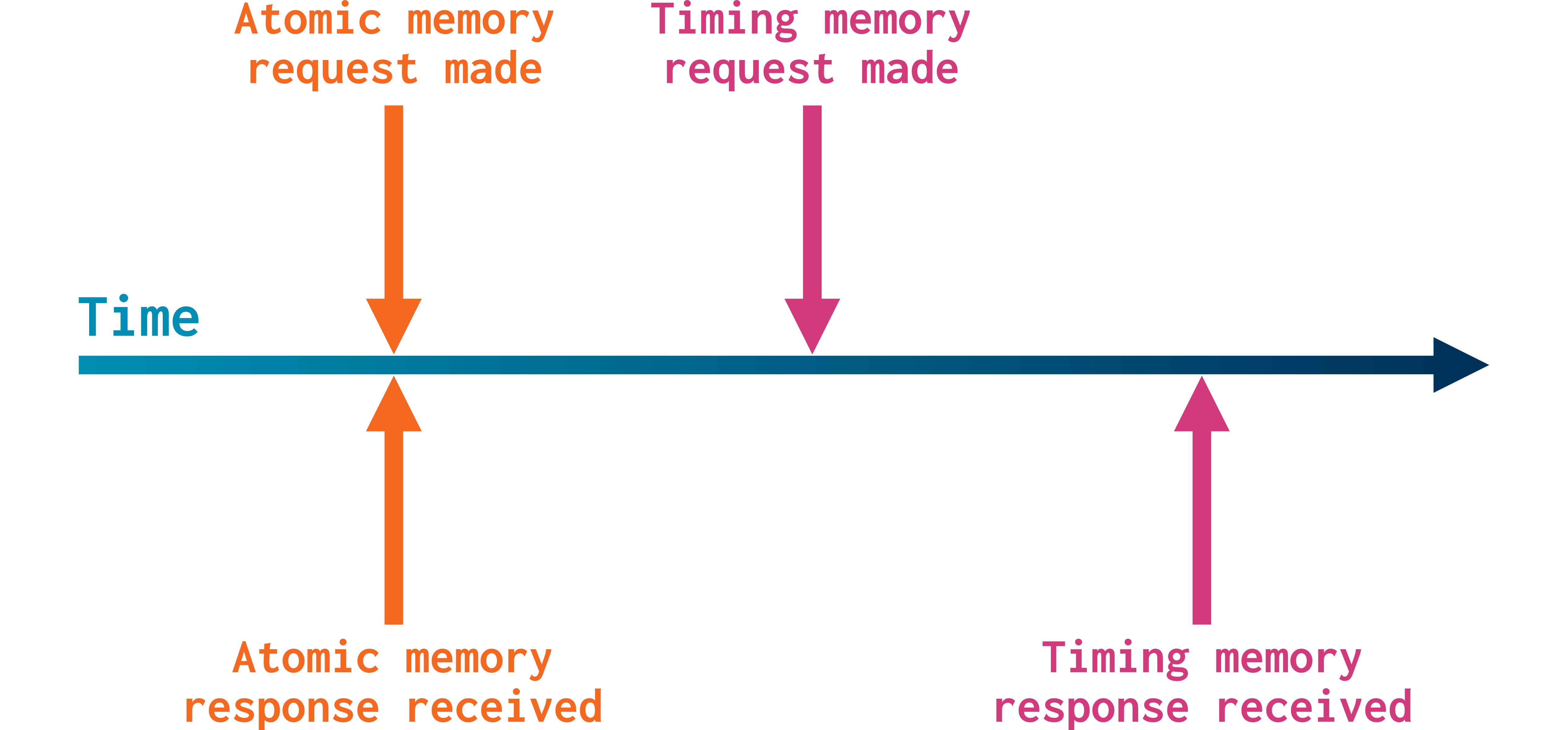
A SimpleCPU interacts with the cache hierarchy when making memory accesses, and it can make memory accesses in three different ways:

• Atomic (performed by BaseAtomicSimpleCPU): atomic memory accesses don’t simulate resource contention or queuing delay. They ignore memory access latency.
  • This makes atomic accesses ideal for fast-forwarding and for warming up caches.
• Timing (performed by BaseTimingSimpleCPU): timing accesses do model resource contention and queuing delay. Responses to memory requests are sent after the simulated memory latency.
  • This means that memory accesses on a BaseTimingSimpleCPU take multiple cycles, while all other non-memory operations take one cycle.
• Functional (used for loading binaries): these are “back door” accesses to memory that have no effect on the cache/memory system’s coherency state.

A SimpleCPU is a good choice for when you aren’t paying too much attention to the processor’s performance, such as when primarily observing memory latency. If you want to simulate more advanced processor features like out-of-order execution or advanced branch prediction, you’ll want a different CPU type.

KVM

KVM stands for “Kernel-based Virtual Machine”. This CPU model allows for native execution on x86 and ARM hosts; basically, using your machine’s actual CPU to execute instructions instead of a simulated CPU model. As you might imagine, this is really fast compared to simulating a CPU. However, it means that the ISA of your host machine has to match the ISA of the simulation. Otherwise, your CPU would have no idea what to do!

We use KVM for fast-forwarding and functional tests, and it’s great for this purpose. That being said, you wouldn’t want to use KVM if you’re trying to collect any meaningful statistics about performance.

Minor CPU

gem5’s minor CPU is an in-order pipelined CPU with the following four stages:

• Fetch1: Handles ITLB (Instruction Translation Lookaside Buffer) accesses and instruction fetch from main memory.
• Fetch2: Decodes instructions.
• Decode: Performs related bookkeeping tasks.
• Execute: Manages instruction issue, execution, memory access, writeback, and commit.

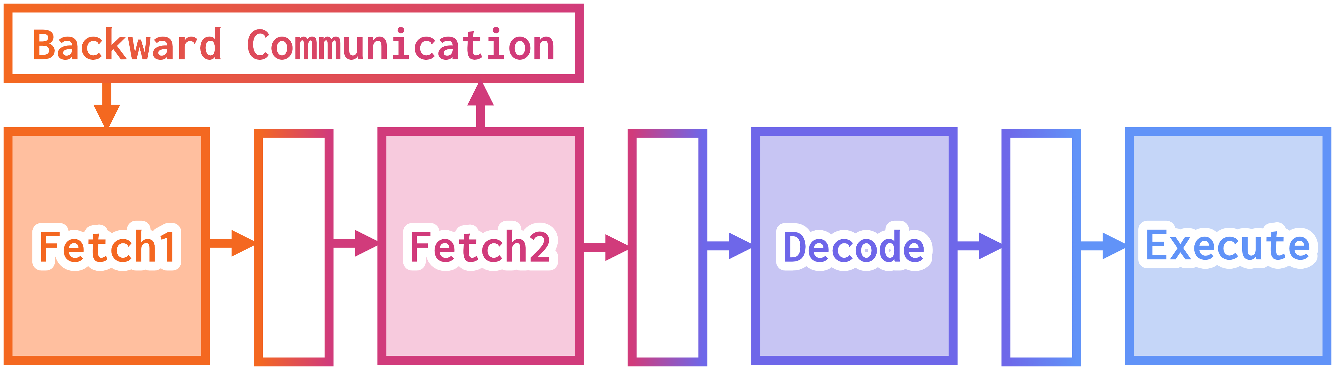
MinorCPU is designed to make the interactions between the pipelined stages of the CPU easier to understand; this means that while its implementation provides a good amount of detail, it is somewhat simplified compared to gem5’s O3 model (which we’ll discuss in a moment).

The minor CPU model makes timing memory accesses and interacts with the cache hierarchy (like BaseTimingSimpleCPU does). It has more robust branch prediction capabilities than the simple CPUs. However, because of its extra simulation detail, it is slower to simulate.

O3 CPU

O3 is shorthand for “out-of-order”. gem5’s O3 processor has five stages:

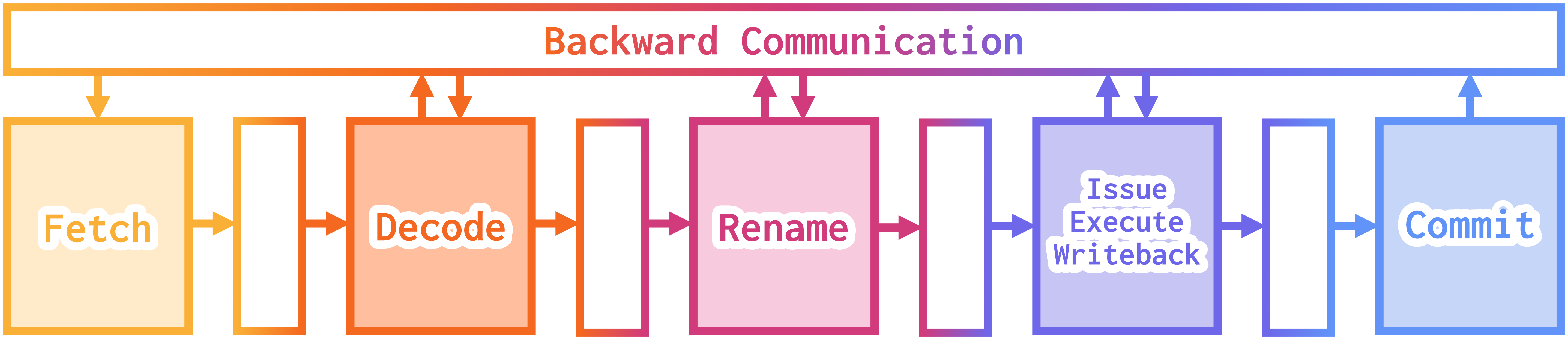
gem5 is an “execute-in-execute” simulator, meaning that instructions executed by gem5’s O3 CPU are executed in the “execute” stage of the pipeline.

Many other simulators (and old gem5 models not discussed here) are not execute-in-execute. This means that they execute instructions either at the beginning or at the end of the pipeline instead, passing the results to a timing backend.

This is an issue for two main reasons: first, if there is an error in the aforementioned timing backend, it won’t show up in the program results; second, instructions cannot be executed out-of-order.

This means that being execute-in-execute uniquely allows us to simulate out-of-order interactions!

Much like the minor CPU, the O3 CPU makes timing memory accesses, interacts with the cache hierarchy, and has detailed branch prediction capabilities. It, too, is slower to simulate. The O3 CPU model is the closest thing to a real CPU provided by gem5 (it’s loosely based on the Alpha 21264!).

Using gem5’s CPU models

To recap, these are the CPU models that exist in gem5:

• BaseAtomicSimpleCPU: A simple CPU model with some branch prediction that makes atomic memory accesses (does not take memory latency into account).
• BaseTimingSimpleCPU: A simple CPU model with some branch prediction that makes timing memory accesses (takes memory latency into account).
• BaseKvmCPU: A KVM (Kernel Virtual Machine) CPU that uses the host’s actual CPU to execute instructions, resulting in really fast execution but unhelpful performance data.
• MinorCPU: An in-order four-stage pipelined CPU with branch prediction capabilities. Slower to simulate.
• O3CPU: An out-of-order five-stage pipelined CPU with branch prediction capabilities. Slower to simulate.

To use any of these CPU models in the cores within gem5’s standard library processor models, set core_type to the appropriate value of the CPUType enum when instantiating a standard library processor:

• CPUTypes.ATOMIC
• CPUTypes.TIMING
• CPUTypes.KVM
• CPUTypes.MINOR
• CPUTypes.O3

We’ve used TIMING CPUs so far in our examples.

Comparing performance

Let’s explore how we can use different CPU core types using standard library components. We’ll be doing the following:

1) Create a system with a cache hierarchy and an ATOMIC CPU. 2) Replace the cache hierarchy with a smaller one and re-simulate. 3) Try both caches with a TIMING CPU instead.

This way, we’ll be able to see how changing our memory access type affects the simulation statistics. Open atomic_vs_timing.py to start.

Currently, this file contains the following:

• A cache hierarchy consisting of a 32-KiB L1 i-cache and d-cache for each core (PrivateL1CacheHierarchy):

cache_hierarchy = PrivateL1CacheHierarchy(
  l1d_size="32KiB", 
  l1i_size="32KiB"
)

• A 1-GiB single-channel DDR3-1600 memory system (SingleChannelDDR3_1600):

memory = SingleChannelDDR3_1600("1GiB")

• A SimpleProcessor with an ATOMIC core type:

cpu_type = CPUTypes.ATOMIC

processor = SimpleProcessor(
  cpu_type=cpu_type,
  isa=ISA.RISCV,
  num_cores=1
)

• A SimpleBoard running a RISC-V matrix multiplication workload:

board = SimpleBoard(
    clk_freq="3GHz",
    processor=processor,
    memory=memory,
    cache_hierarchy=cache_hierarchy
)

workload = obtain_resource("riscv-matrix-multiply-run")
board.set_workload(workload)

The first thing we want to do is run this simulation and save the output in a directory named atomic-normal-cache. We can do that with the following command:

gem5 --outdir=atomic-normal-cache atomic_vs_timing.py

The --outdir flag changes the name of the output directory from the default output directory name (m5out) to a name of your choosing.

Now, let’s shrink the cache and try again:

Your turn: Change the size of the i-cache and d-cache to 1 KiB and rerun the simulation. Save the results in a directory called atomic-small-cache.

Answer

cache_hierarchy = PrivateL1CacheHierarchy(
  l1d_size="1KiB",
  l1i_size="1KiB"
 )

gem5 --outdir=atomic-small-cache atomic_vs_timing.py

Let’s keep the cache how it is but change the CPU type from ATOMIC to TIMING.

Your turn: Change the CPU type to TIMING and rerun the simulation. Save the results in a directory named timing-small-cache.

Answer

cpu_type = CPUTypes.TIMING

gem5 --outdir=timing-small-cache atomic_vs_timing.py

Lastly, let’s put the cache back at 32 KiB.

Your turn: Change the size of the i-cache and d-cache back to 32 KiB and rerun the simulation. Save the results in a directory called timing-normal-cache.

Answer

cache_hierarchy = PrivateL1CacheHierarchy(
 l1d_size="32KiB",
 l1i_size="32KiB"
)

gem5 --outdir=timing-normal-cache atomic_vs_timing.py

Now, let’s compare the results! We’ll find everything we need in stats.txt within the output directories. First, let’s prove that all four of these simulations simulated the same number of ops. We can do this by checking the simOps statistic at the top of stats.txt, either by searching the file by hand or by using the grep command in the terminal:

grep -r 'simOps' <path-to-output-directories>

If you have not seen it before, grep is a command-line utility that searches for text within files. It’s useful for navigating large directories, including the gem5 directory! The -r flag (for “recursive”) specifies that grep should look inside directories, which allows it to find the stat.txt files inside each of output directories we created. We tell it to look for the text string simOps, which conveniently only shows up as the statistic we’re looking for.

Here are the results:

atomic-normal-cache:

simOps                                       33954687

atomic-small-cache:

simOps                                       33954687

timing-normal-cache:

simOps                                       33954687

timing-small-cache:

simOps                                       33954687

Running the same workload on the same configuration yields the same number of ops, which makes sense; we kept the workload, which determines the instructions being executed, exactly the same, and the cores only changed their memory access mode. Note that the number of ops may not be the exact same as the number of instructions, since gem5 breaks down some instructions into micro-ops.

Now for our experiment: how many CPU cycles were required to multiply these matrices? We can find this out using the numCycles statistic, which is collected for each core and tracks the total number of CPU cycles simulated.

Your turn: Write a grep command to search for the numCycles statistic in the output directories for our cache simulations.

Answer

grep -r 'numCycles' <path-to-output-directories>

atomic-normal-cache:

board.processor.cores.core.numCycles        38157732 

atomic-small-cache:

board.processor.cores.core.numCycles        38157732 

timing-normal-cache:

board.processor.cores.core.numCycles        62830921 

timing-small-cache:

board.processor.cores.core.numCycles        112602851

You may notice that the timing CPU executed for more simulated cycles than the atomic CPU on the same cache size. This is because any memory accesses we make take longer on a timing CPU compared to an atomic CPU. More interestingly, you’ll notice that for the atomic CPU, the number of CPU cycles didn’t change when we switched our cache models! Since atomic memory accesses don’t take memory latency into account, the fact that our cache was smaller (and thus that we accessed memory more often) made no difference. The difference is clear for the timing CPU, however, where the smaller cache significantly increased the number of simulated cycles.

If you’d like, you can change the CPU type again to O3 and take a look at the results!

Keep these results in mind when selecting which CPU type is approriate for your gem5 simulations. Some kind of timing CPU is the right choice if memory access latency matters to your work.

Creating custom processor components

We can do better than just using CPU models in standard library components. We can create our own components!

Changing model parameters with extension

gem5 models have a lot of parameters. For example, here are just a few of the parameters for BaseO3CPU:

decodeToFetchDelay = Param.Cycles(1, "Decode to fetch delay")
renameToFetchDelay = Param.Cycles(1, "Rename to fetch delay")
iewToFetchDelay = Param.Cycles(1, "Issue/Execute/Writeback to fetch delay")
commitToFetchDelay = Param.Cycles(1, "Commit to fetch delay")
fetchWidth = Param.Unsigned(8, "Fetch width")
fetchBufferSize = Param.Unsigned(64, "Fetch buffer size in bytes")

These parameters (and many more) can be found in src/cpu/o3/BaseO3CPU.py. Don’t worry too much about this syntax for now! We’ll talk about what this means when we cover how to create gem5 models in the next unit.

In this snippet, we can see the following:

• The decode-to-fetch delay with a value of 1 cycle,
• The rename-to-fetch delay with a value of 1 cycle,
• The issue/execute/writeback-to-fetch delay with a value of 1 cycle,
• The commit-to-fetch delay with a value of 1 cycle,
• The fetch width with a value of 8 instructions,
• The fetch buffer size with a value of 64 bytes.

The way we change these parameters’ values in our code is not by changing this file, or even by directly creating an instance of this component in our code. We customize parameter values of gem5 components by extending their classes in Python.

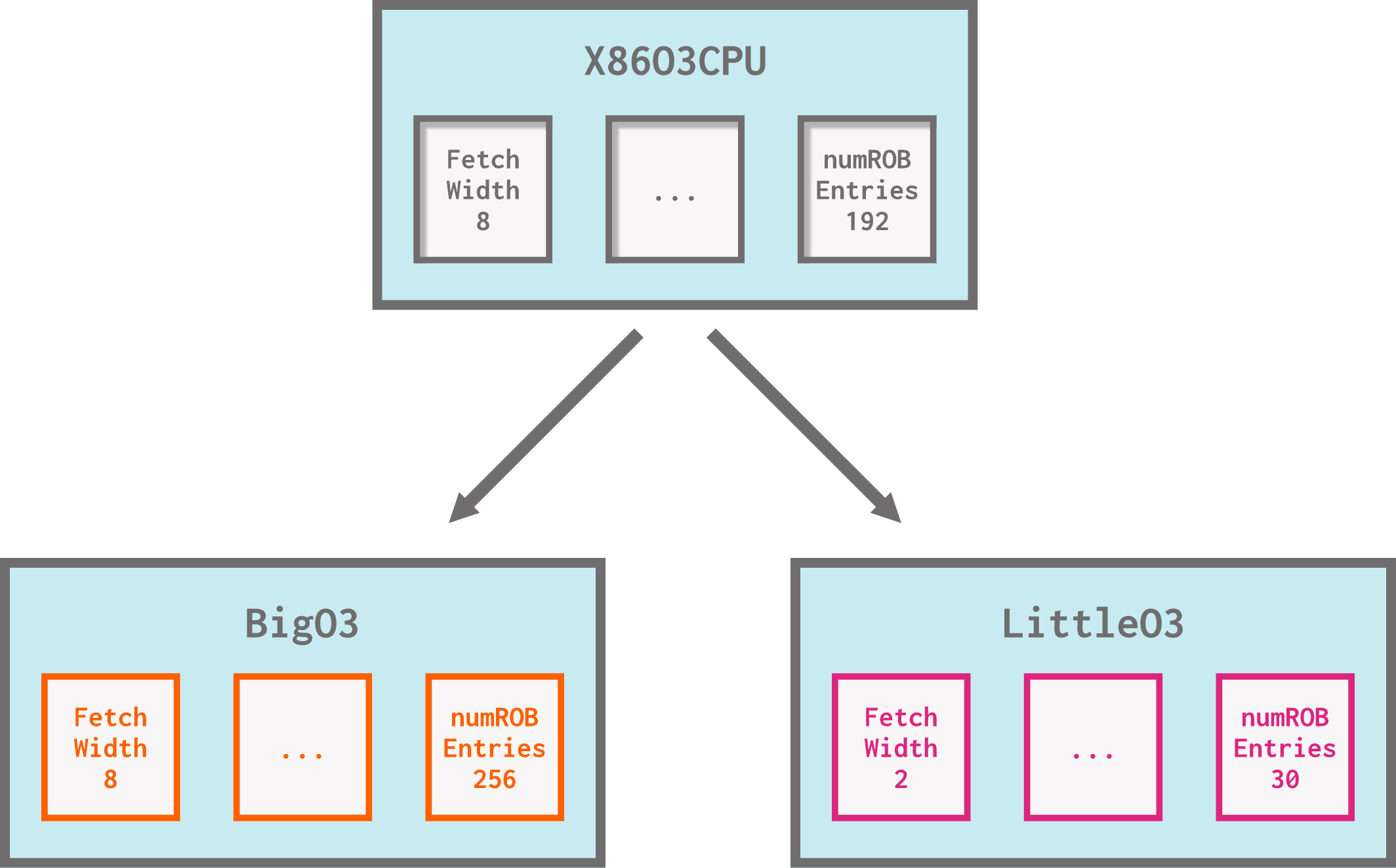
Let’s see this in action by starting to create our very own processor. For this example, we’ll be extending one of gem5’s out-of-order CPU models, X86O3CPU. Open my_processors.py to get started. Currently, this file is mostly empty! We’ll be defining our O3 CPUs with custom parameters here.

First, let’s create BigO3, an O3 CPU with… big parameters! We’ll specifically be doing the following:

• Setting the fetch, decode, rename, dispatch, issue, writeback, and commit widths to 8 bytes,
• Setting the number of ROB (re-order buffer) entries to 256,
• Setting the number of physical int and float registers to 512.

O3 CPUs in gem5 are ISA-specific. Therefore, we’ll we extending X86O3CPU instead of just BaseO3CPU.

Let’s create the BigO3 class and set all of these parameters:

class BigO3(RiscvO3CPU):
    def __init__(self):
        super().__init__()
        self.fetchWidth = 8
        self.decodeWidth = 8
        self.renameWidth = 8
        self.dispatchWidth = 8
        self.issueWidth = 8
        self.wbWidth = 8
        self.commitWidth = 8

        self.numROBEntries = 256
        self.numPhysIntRegs = 512
        self.numPhysFloatRegs = 512

We also want another core type with little parameters to compare BigO3 to. We want a CPU that has the following:

• Fetch, decode, rename, dispatch, issue, writeback, and commit widths set to 2 bytes,
• Number of ROB (re-order buffer) entries set to 30,
• The number of physical int and float registers set to 80.

Your turn: Write the LittleO3 class to set the parameters above to our desired values.

Answer

class LittleO3(X86O3CPU):
    def __init__(self):
        super().__init__()
        self.fetchWidth = 2
        self.decodeWidth = 2
        self.renameWidth = 2
        self.dispatchWidth = 2
        self.issueWidth = 2
        self.wbWidth = 2
        self.commitWidth = 2

        self.numROBEntries = 30
        self.numPhysIntRegs = 80
        self.numPhysFloatRegs = 80

We’ve now created our custom CPU models to use in the cores of our processor!

Wrapping models with components

Great, now we have some customized parameters for our CPU models… but how do we use them? In order for these models to be useful, we need to wrap them in a standard library core component.

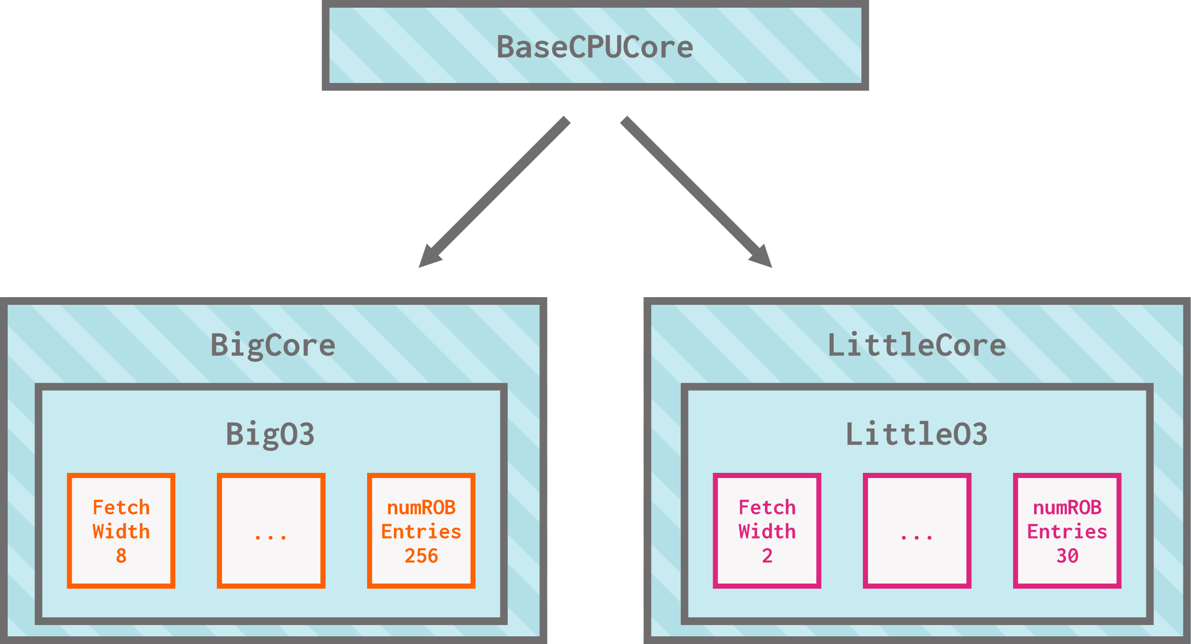
The best standard library component to inherit from to make our wrapper component is BaseCPUCore. This is the parent class of SimpleCore, which you may remember as the core used by SimpleProcessor and SwitchableProcessor. BaseCPUCore provides the standard interface for CPU cores. Thankfully, it’s super straightforward to extend BaseCPUCore!

In the same my_processors.py file, we can now add two new classes, BigCore and LittleCore. As the names suggest, BigCore will wrap around BigO3 and LittleCore will wrap around LittleO3. All we need to add these classes is:

1) Extend BaseCPUCore, 2) Create a core of our custom type, 3) Call our parent’s __init__ with the core and the appropriate ISA.

class BigCore(BaseCPUCore):
    def __init__(self):
        core = BigO3()
        super().__init__(core, ISA.X86)

Your turn: Write the LittleCore class to wrap LittleO3 in a standard library core.

Answer

class LittleCore(BaseCPUCore):
    def __init__(self):
        core = LittleO3()
        super().__init__(core, ISA.X86)

Sweet! Now we have some standard library cores. Next, a processor.

Building the processor

To use our shiny new standard library cores, we need to put them inside of a standard library processor (which can plug into a board!).

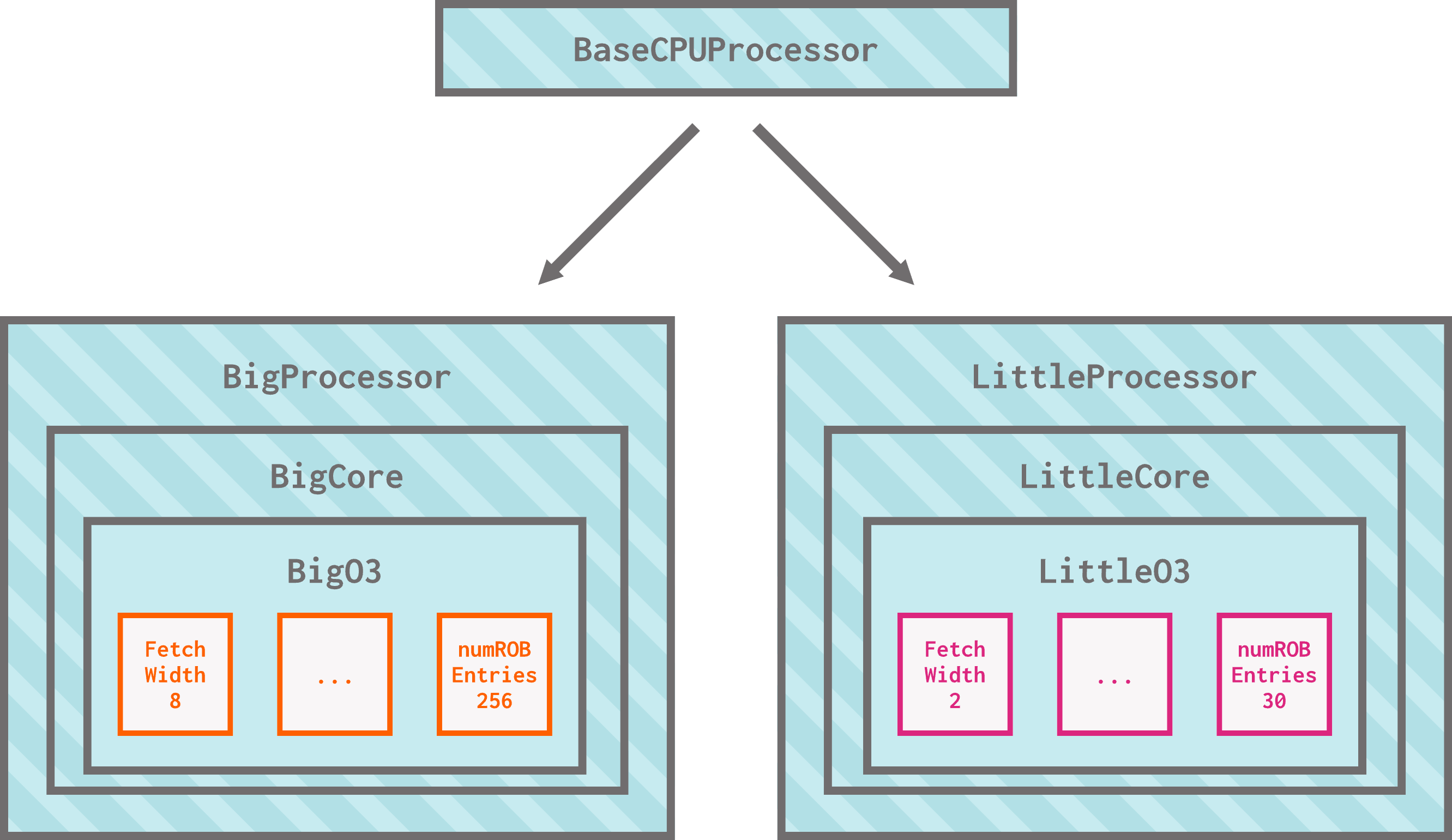
The best class to inherit from to create our standard library processor is BaseCPUProcessor, which is the parallel to BaseCPUCore in processor land. This is the parent class to SimpleProcessor. Once again, it’s very straightforward to extend BaseCPUProcessor.

In the same my_processors.py file, we can add our final two classes: BigProcessor and LittleProcessor. For each class, we need to:

1) Extend from BaseCPUProcessor, 2) Create a list of cores of the appropriate type, 3) Pass the list to the parent’s __init__.

class BigProcessor(BaseCPUProcessor):
    def __init__(self):
        core_list = [BigCore()]
        super().__init__(
            cores = core_list
        )

Your turn: Write the LittleProcessor class to pass a single LittleCore into a standard library processor.

Answer

class LittleProcessor(BaseCPUProcessor):
    def __init__(self):
        core_list = [LittleCore()]
        super().__init__(
            cores = core_list
        )

And that, finally, is it!

Let’s run this thing!

Let’s recap everything we just did:

1) From base CPU model to specialized CPU models: We extended the X86O3CPU class to change its parameter values, creating BigO3 and LittleO3. 2) From CPU models to cores: We wrapped the BigO3 and LittleO3 models with matching standard library components, BigCore and LittleCore, which extend BaseCPUCore. 3) From cores to processors: We passed our newly-created standard library cores into newly-created standard library processors, BigProcessor and LittleProcessor, which extend BaseCPUProcessor.

What we’re left with are two new standard library processors containing cores with our chosen custom parameters.

There are quite a few more parameters available in BaseO3CPU that we didn’t touch, so the customization options are even more expansive than what this example shows!

We can now take BigProcessor and LittleProcessor and plug them into a standard library board just like we did with SimpleProcessor in our previous example. In fact, let’s put them in our hello world example! A copy of stdlib_hello_world.py (with the modifications made in the last section) named hello_processors.py is provided for convenience.

The workspace directory is organized such that the configuration script is able to find our new components in its search path. If this is not the case in your future work, note that the Python search path must be expanded to include the location of the file(s) definining new components, which can be done with import sys and sys.path.append(<path>).

Remove the ISA and CPUTypes imports and replace the import statement for SimpleProcessor with the following:

from my_processors import BigProcessor, LittleProcessor

Next, we can swap out the processor for our new processors! Let’s use LittleProcessor first:

processor = LittleProcessor()

Let’s compare these CPUs on a more interesting workload than the first 20 milliseconds of booting Ubuntu. Swap out "x86-ubuntu-24.04-boot-no-systemd" in the call to obtain_resource with x86-matrix-multiply-run:

board.set_workload(
    obtain_resource("x86-matrix-multiply-run")
)

Additionally, remove the 20 millisecond restriction on simulation time by removing the parameter to sim.run(20_000_000_000):

sim.run()

That’s it! We can now run this script. Let’s redicrect its output to a directory named little-o3 so we can compare our results later:

gem5 --outdir=little-o3 hello_processors.py 

Your turn: Switch out LittleProcessor for BigProcessor and run the simulation again, redirecting the output to a directory named big-o3.

Answer

processor = BigProcessor()

gem5 --outdir=big-o3 hello_processors.py 

You should see some changes in the simulation statistics. Let’s look at how long the simulation took, as well as how many CPU cycles were simulated.

Your turn: Search for the simSeconds and numCycles statistics in the little-o3 and big-o3 output directories.

Answer

grep -r 'simSeconds' <path-to-output-directories>

grep -r 'numCycles' <path-to-output-directories>

You should see the following:

little-o3:

simSeconds                                   0.010227 
board.processor.cores.core.numCycles         30713015  

big-o3:

simSeconds                                   0.009471 
board.processor.cores.core.numCycles         28440669

As we might expect, BigProcessor is able to execute the workload in fewer simulated cycles and thus in fewer simulation seconds.

There are a lot more things to explore when it comes to processors in gem5! If you’re looking to learn about more advanced features in the context of processors, take the processor track in Unit IV!